This week 010 post is about how to use Tableau Prep to manipulate the below three tables(showing first 5 only),
| Liquid | Bar | Sign-up Date | |
| dmalone1@tumblr.com | 1 | 0 | 14/01/2016 |
| dsworder6@is.gd | 0 | 1 | 11/12/2016 |
| bandresen8@rakuten.co.jp | 1 | 1 | 07/11/2016 |
| cmiskin9@dion.ne.jp | 1 | 1 | 30/07/2017 |
| tmenguyb@people.com.cn | 0 | 1 | 30/10/2016 |
| first_name | last_name | Date |
| Donielle | Malone | 23.04.2018 |
| Dorry | Sworder | 26.12.2018 |
| Benedict | Andresen | 24.12.2018 |
| Cornell | Miskin | 10.12.2018 |
| Theresita | Menguy | 28.08.2018 |
| Liquid Sales to Date | Bar Sales to Date | |
| dmalone1@tumblr.com | 9380 | 3927 |
| dsworder6@is.gd | 8731 | 4300 |
| bandresen8@rakuten.co.jp | 9655 | 611 |
| cmiskin9@dion.ne.jp | 8371 | 1814 |
| tmenguyb@people.com.cn | 567 | 1300 |
to the below two formatted tables.
| Status | Interested in Liquid Soap | Interested In Soap Bars | Sign-up Date | Unsubscribe Date | Liquid Sales to Date | Bar Sales to Date | |
| Resubscribed | esooleyd@pcworld.com | 1 | 0 | 3/12/2018 | 28/04/2018 | 6248 | 4716 |
| Resubscribed | mizkovicir@cyberchimps.com | 1 | 0 | 26/12/2018 | 17/07/2018 | 4735 | 4687 |
| Resubscribed | etyres3p@archive.org | 1 | 0 | 14/10/2018 | 8/8/2018 | 2225 | 4701 |
| Resubscribed | fcatonne40@studiopress.com | 0 | 1 | 20/09/2018 | 20/05/2018 | 7244 | 2690 |
| Resubscribed | cguiduzzi5i@plala.or.jp | 1 | 1 | 19/06/2018 | 24/05/2018 | 8056 | 3454 |
| Resubscribed | bmatisoff5j@flickr.com | 1 | 0 | 20/12/2018 | 4/10/2018 | 4873 | 1186 |
| Subscribed | pvenart0@posterous.com | 1 | 0 | 16/08/2018 | 159 | 1723 | |
| Subscribed | erosedale2@google.com.hk | 0 | 1 | 13/01/2016 | 2019 | 3452 | |
| Subscribed | obowman3@hubpages.com | 1 | 0 | 11/11/2018 | 6943 | 422 | |
| Subscribed | fmacpadene4@behance.net | 1 | 1 | 19/07/2017 | 8937 | 1569 |
| Months before Unsubscribed group | Status | Interested in Liquid Soap | Interested In Soap Bars | Liquid Sales to Date | Bar Sales to Date | |
| 0-3 | Unsubscribed | 1 | 0 | 3 | 18419 | 5865 |
| 24+ | Unsubscribed | 1 | 0 | 13 | 63415 | 34082 |
| Resubscribed | 1 | 1 | 1 | 8056 | 3454 | |
| 24+ | Unsubscribed | 0 | 1 | 11 | 56639 | 29523 |
| Subscribed | 0 | 1 | 34 | 144420 | 81908 | |
| 6-Mar | Unsubscribed | 0 | 1 | 2 | 3927 | 6190 |
| 6-Mar | Unsubscribed | 1 | 0 | 3 | 19665 | 11449 |
| Resubscribed | 1 | 0 | 4 | 18081 | 15290 | |
| Subscribed | 1 | 1 | 26 | 141973 | 64129 | |
| 6-Mar | Unsubscribed | 1 | 1 | 5 | 25420 | 9041 |
On the input file, there are three tabs, [Mailing List 2018] , [Unsubscribe list], and [Customer Lifetime Value].
The idea of this exercise is to:
- Combine these two tables [Mailing List 2018] and [Unsubscribe list] together into one table using full join to filter for subscribed and resubscribed members
- Combine the subscribed and resubscribed members with this table [Customer Lifetime Value]
- The purpose is to generate a table with the total liquid and bar sales
- Generate a table that bin the months before unsubscribed into the following group based on the months difference between Sign-Up Date and Unsubscribed Date
- 0 – 3
- 3 – 6
- 6 – 12
- 12 – 24
- +24 =
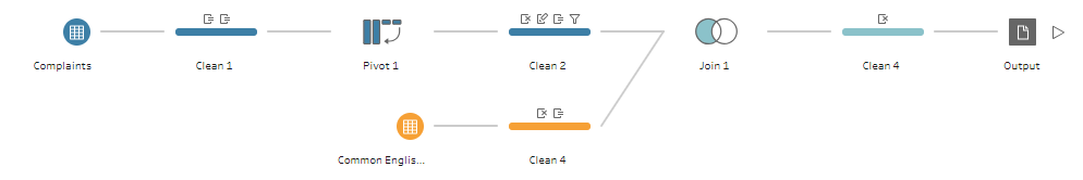
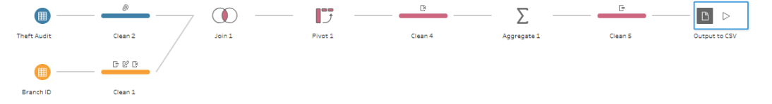
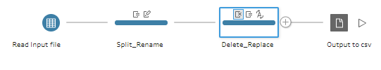
As shown on the below image, here are the steps to create the above output file.
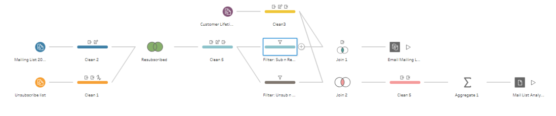
Below are the steps to create the above tables.
- Read the input file by drag and drop this table [Mailing List 2018]
- Add another step for data cleaning
- Select the [email] field and click on Custom Split
- On Split off, select First and 1
- On Use the separator, enter @
- Add the Remove_last_letter field with this formula
- left([email – Split 1],LEN([email – Split 1])-1)
- This is to remove the last letter
- Remove numbers by selecting Clean > Remove Numbers
- Rename [Remove_last_letter] as JoinField
- This is to use this field as join with the {Unsubscribe list]]
- Select the [email] field and click on Custom Split
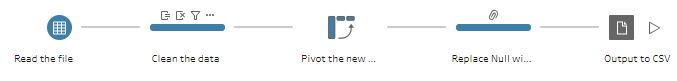
- Read the input file by drag and drop this table [Unsubscribe list]
- Add another step for data cleaning
- Add the [First _letter] with this formula
- lower(LEFT([first_name], 1))
- This is to extract the first letter only
- Remove the [First_name] field
- lower(LEFT([first_name], 1))
- Change the [Date] field as Date
- Add the [JoinField] field with this formula
- lower([First_Letter]+[last_name])
- This is to use this field as join with the {Mailing List 2018]
- Remove punctuation by selecting Clean > Remove Numbers
- Remove all spaces by selecting Clean > Remove All Spaces
- Remove both [First_letter] and [Last_name]
- Add the [First _letter] with this formula
- Drag Clean1 to Clean2
- On Applied Join clauses, select JoinField for both sides
- On Join Type, make it Full Join
- Add another step for data cleaning
- Remove the following both fields
- [email-split1] and {JoinFiled-1]
- Rename [Date] to [Unsubscribed Date]
- Rename [Liquid] to [Interested in Soap Bars]
- Rename [Bar] to [Interested in Soap Bars]
- Add the [status] field with this formula
- IF ISNULL([Unsubscribed Date]) THEN ‘Subscribed’
ELSEIF [Sign-up Date] >= [Unsubscribed Date] THEN “Resubscribed”
ELSE “Unsubscribed”
END
- IF ISNULL([Unsubscribed Date]) THEN ‘Subscribed’
- Remove the following both fields
- Add another step to filter for subscriber and resubscriber
- Click on the [Status] field and select Filter Values
- On the Filter, select both Resubscribed and Subscribed
- Drag the [Customer Lifetime] table to the Canvas
- Add another step for data cleaning
- Copy what is on the clean2 step to clean 3 steps
- Add another step for data cleaning
- Drag the filter: Sub n Resub step to clean 3 to inner join it based on the JoinField
- Add the output step to create the [Email List with Detail]
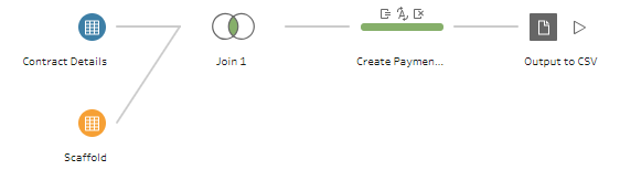
- To create the [Mail List Analytics] table, follow these steps
- On the clean5 step, click to add a branch
- On the [status] filter, make sure all selections are selected
- Drag the [Filter All] step to [clean3] step to inner join based on the JoinField
- Add another step for data cleaning
- Create this field [Month Dif] for the month difference calculation
- DATEDIFF(‘month’,[Sign-up Date],[Unsubscribed Date])
- Add this field [Months before Unsubscribed Group] with this formula
- IF [Month DIF] >= 24 THEN “24+”
ELSEIF [Month DIF] >= 12 THEN “12-24”
ELSEIF [Month DIF] >= 6 THEN “6-12”
ELSEIF [Month DIF] >= 3 THEN “3-6”
ELSEIF [Month DIF] >= 0 THEN “0-3”
ELSE “”
END - This will be use for grouping
- IF [Month DIF] >= 24 THEN “24+”
- Create this field [Month Dif] for the month difference calculation
- Remove the following fields
- [Unsubscribed Date
- [Sign-Up Date]
- [JoinField]
- [JoinField-1]
- {Month Dif]
- Add an Aggregate step
- Drag these fields to group fields
- [Momths Before Unsubscribed Group]
- {Interested in Liquid Soap]
- Interested in Soap Bars
- [Status]
- Drag these fields to aggregate fields
- [Liquid Sales to Date]
- Bar Sales to Date
- [meail]
- make this as CNT, which is for count
- Drag these fields to group fields
- add the output step to create the [Mail List Analytics]
- On the clean5 step, click to add a branch
Attached is the Week 010 Solution.tflx.
The input file is from the following site, https://preppindata.blogspot.com.
I encourage you to follow that site to learn about Tableau Prep.